Introduction and Review of Thermodynamics
How to Study Chem 1.0.1 More Effectively

1.1 Spontaneity
Learning Objectives
By the end of this section, you will be able to:
- Distinguish between spontaneous and nonspontaneous processes
- Describe the dispersal of matter and energy that accompanies certain spontaneous processes
Processes have a natural tendency to occur in one direction under a given set of conditions. Water will naturally flow downhill but uphill flow requires outside intervention such as the use of a pump. Iron exposed to the earth’s atmosphere will corrode but rust is not converted to iron without intentional chemical treatment. A spontaneous process is one that occurs naturally under certain conditions. A nonspontaneous process on the other hand, will not take place unless it is “driven” by the continual input of energy from an external source. A process that is spontaneous in one direction under a particular set of conditions is nonspontaneous in the reverse direction. At room temperature and typical atmospheric pressure, for example, ice will spontaneously melt but water will not spontaneously freeze.
The spontaneity of a process is not correlated to the speed of the process. A spontaneous change may be so rapid that it is essentially instantaneous or so slow that it cannot be observed over any practical period of time. To illustrate this concept, consider the decay of radioactive isotopes, a topic more thoroughly treated in the chapter on nuclear chemistry. Radioactive decay is by definition a spontaneous process in which the nuclei of unstable isotopes emit radiation as they are converted to more stable nuclei. All the decay processes occur spontaneously but the rates at which different isotopes decay vary widely. Technetium-99m is a popular radioisotope for medical imaging studies that undergoes relatively rapid decay and exhibits a half-life of about six hours. Uranium-238 is the most abundant isotope of uranium and its decay occurs much more slowly exhibiting a half-life of more than four billion years (Figure 1.1).
Figure 1.1
Both U-238 and Tc-99m undergo spontaneous radioactive decay, but at drastically different rates. Over the course of one week, essentially all of a Tc-99m sample and none of a U-238 sample will have decayed.

As another example, consider the conversion of diamond into graphite (Figure 1.2).
The phase diagram for carbon indicates that graphite is the stable form of this element under ambient atmospheric pressure while diamond is the stable allotrope at very high pressures such as those present during its geologic formation. Thermodynamic calculations of the sort described in the last section of this chapter indicate that the conversion of diamond to graphite at ambient pressure occurs spontaneously yet diamonds are observed to exist, and persist, under these conditions. Though the process is spontaneous under typical ambient conditions, its rate is extremely slow; so, for all practical purposes diamonds are indeed “forever.” Situations such as these emphasize the important distinction between the thermodynamic and the kinetic aspects of a process. In this particular case, diamonds are said to be thermodynamically unstable but kinetically stable under ambient conditions.
Figure 1.2
The conversion of carbon from the diamond allotrope to the graphite allotrope is spontaneous at ambient pressure, but its rate is immeasurably slow at low to moderate temperatures. This process is known as graphitization and its rate can be increased to easily measurable values at temperatures in the 1000–2000 K range. (credit "diamond" photo: modification of work by "Fancy Diamonds"/Flickr; credit "graphite" photo: modification of work by images-of-elements.com/carbon.php)

1.1.1 Dispersal of Matter and Energy
Extending the discussion of thermodynamic concepts toward the objective of predicting spontaneity, consider now an isolated system consisting of two flasks connected with a closed valve. Initially there is an ideal gas in one flask and the other flask is empty (P = 0). (Figure 1.3). When the valve is opened, the gas spontaneously expands to fill both flasks equally. Recalling the definition of pressure-volume work from the chapter on thermochemistry note that no work has been done because the pressure in a vacuum is zero.
Note as well that since the system is isolated, no heat has been exchanged with the surroundings (q = 0). The first law of thermodynamics confirms that there has been no change in the system’s internal energy as a result of this process.
The spontaneity of this process is therefore not a consequence of any change in energy that accompanies the process. Instead, the driving force appears to be related to the greater, more uniform dispersal of matter that results when the gas is allowed to expand. Initially, the system was comprised of one flask containing matter and another flask containing nothing. After the spontaneous expansion took place, the matter was distributed both more widely (occupying twice its original volume) and more uniformly (present in equal amounts in each flask).
Figure 1.3
An isolated system consists of an ideal gas in one flask that is connected by a closed valve to a second flask containing a vacuum. Once the valve is opened, the gas spontaneously becomes evenly distributed between the flasks.

Now consider two objects at different temperatures: object X at temperature TX and object Y at temperature TY, with TX > TY (Figure 1.4). When these objects come into contact, heat spontaneously flows from the hotter object (X) to the colder one (Y). This corresponds to a loss of thermal energy by X and a gain of thermal energy by Y.
From the perspective of this two-object system, there was no net gain or loss of thermal energy, rather the available thermal energy was redistributed among the two objects. This spontaneous process resulted in a more uniform dispersal of energy.
Figure 1.4
When two objects at different temperatures come in contact, heat spontaneously flows from the hotter to the colder object.

As illustrated by the two processes described, an important factor in determining the spontaneity of a process is the extent to which it changes the dispersal or distribution of matter and/or energy. In each case, a spontaneous process took place that resulted in a more uniform distribution of matter or energy.
EXAMPLE 1.1.2
Redistribution of Matter during a Spontaneous Process
Describe how matter is redistributed when the following spontaneous processes take place:
(a) A solid sublimes.
(b) A gas condenses.
(c) A drop of food coloring added to a glass of water forms a solution with uniform color.
Solution
Figure 1.5
(credit a: modification of work by Jenny Downing; credit b: modification of work by “Fuzzy Gerdes”/Flickr; credit c: modification of work by Paul A. Flowers)

(a) Sublimation is the conversion of a solid (relatively high density) to a gas (much lesser density). This process yields a much greater dispersal of matter, since the molecules will occupy a much greater volume after the solid-to-gas transition.
(b) Condensation is the conversion of a gas (relatively low density) to a liquid (much greater density). This process yields a much lesser dispersal of matter, since the molecules will occupy a much lesser volume after the gas-to-liquid transition.
(c) The process in question is diffusion. This process yields a more uniform dispersal of matter since the initial state of the system involves two regions of different dye concentrations (high in the drop of dye, zero in the water), and the final state of the system contains a single dye concentration throughout.
Check Your Learning
Describe how energy is redistributed when a spoon at room temperature is placed in a cup of hot coffee.
Answer
Heat will spontaneously flow from the hotter object (coffee) to the colder object (spoon), resulting in a more uniform distribution of thermal energy as the spoon warms and the coffee cools.
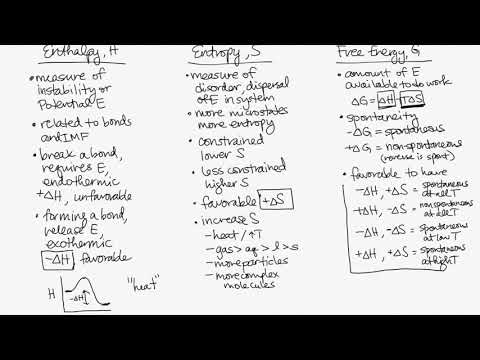
1.2 Entropy
Learning Objectives
By the end of this section, you will be able to:
- Define entropy
- Explain the relationship between entropy and the number of microstates
- Predict the sign of the entropy change for chemical and physical processes
In 1824, at the age of 28, Nicolas Léonard Sadi Carnot (Figure 1.6) published the results of an extensive study regarding the efficiency of steam heat engines. A later review of Carnot’s findings by Rudolf Clausius introduced a new thermodynamic property that relates the spontaneous heat flow accompanying a process to the temperature at which the process takes place. This new property was expressed as the ratio of the reversible heat (qrev) and the kelvin temperature (T). In thermodynamics, a reversible process is one that takes place at such a slow rate that it is always at equilibrium and its direction can be changed (it can be “reversed”) by an infinitesimally small change in some condition. Note that the idea of a reversible process is a formalism required to support the development of various thermodynamic concepts; no real processes are truly reversible rather they are classified as irreversible.
Figure 1.6
(a) Nicholas Léonard Sadi Carnot’s research into steam-powered machinery and (b) Rudolf Clausius’s later study of those findings led to groundbreaking discoveries about spontaneous heat flow processes.

Similar to other thermodynamic properties, this new quantity is a state function so its change depends only upon the initial and final states of a system. In 1865, Clausius named this property entropy (S) and defined its change for any process as the following:
The entropy change for a real, irreversible process is then equal to that for the theoretical reversible process that involves the same initial and final states.
1.2.1 Entropy and Microstates
Following the work of Carnot and Clausius, Ludwig Boltzmann developed a molecular-scale statistical model that related the entropy of a system to the number of microstates (W) possible for the system. A microstate is a specific configuration of all the locations and energies of the atoms or molecules that make up a system. The relation between a system’s entropy and the number of possible microstates is
where k is the Boltzmann constant, 1.38 10−23 J/K.
As for other state functions, the change in entropy for a process is the difference between its final (Sf) and initial (Si) values:
For processes involving an increase in the number of microstates, Wf > Wi, the entropy of the system increases and ΔS > 0. Conversely, processes that reduce the number of microstates, Wf < Wi, yield a decrease in system entropy, ΔS < 0. This molecular-scale interpretation of entropy provides a link to the probability that a process will occur as illustrated in the next paragraphs.
Consider the general case of a system comprised of N particles distributed among n boxes. The number of microstates possible for such a system is nN. For example, distributing four particles among two boxes will result in 24 = 16 different microstates as illustrated in Figure 1.7. Microstates with equivalent particle arrangements (not considering individual particle identities) are grouped together and are called distributions. The probability that a system will exist with its components in a given distribution is proportional to the number of microstates within the distribution. Since entropy increases logarithmically with the number of microstates, the most probable distribution is therefore the one of greatest entropy.
Figure 1.7
The sixteen microstates associated with placing four particles in two boxes are shown. The microstates are collected into five distributions—(a), (b), (c), (d), and (e)—based on the numbers of particles in each box.

For this system, the most probable configuration is one of the six microstates associated with distribution (c) where the particles are evenly distributed between the boxes, that is, a configuration of two particles in each box. The probability of finding the system in this configuration is or The least probable configuration of the system is one in which all four particles are in one box, corresponding to distributions (a) and (e), each with a probability of The probability of finding all particles in only one box (either the left box or right box) is then or
As you add more particles to the system, the number of possible microstates increases exponentially (2N). A macroscopic (laboratory-sized) system would typically consist of moles of particles (N ~ 1023), and the corresponding number of microstates would be staggeringly huge. Regardless of the number of particles in the system, however, the distributions in which roughly equal numbers of particles are found in each box are always the most probable configurations.
This matter dispersal model of entropy is often described qualitatively in terms of the disorder of the system. By this description, microstates in which all the particles are in a single box are the most ordered thus possessing the least entropy. Microstates in which the particles are more evenly distributed among the boxes are more disordered possessing greater entropy.
The previous description of an ideal gas expanding into a vacuum (Figure 1.3) is a macroscopic example of this particle-in-a-box model. For this system the most probable distribution is confirmed to be the one in which the matter is most uniformly dispersed or distributed between the two flasks. Initially, the gas molecules are confined to just one of the two flasks. Opening the valve between the flasks increases the volume available to the gas molecules and, correspondingly, the number of microstates possible for the system. Since Wf > Wi, the expansion process involves an increase in entropy (ΔS > 0) and is spontaneous.
A similar approach may be used to describe the spontaneous flow of heat. Consider a system consisting of two objects, each containing two particles, and two units of thermal energy (represented as “*”) in Figure 1.8. The hot object is comprised of particles A and B and initially contains both energy units. The cold object is comprised of particles C and D, which initially has no energy units. Distribution (a) shows the three microstates possible for the initial state of the system, with both units of energy contained within the hot object. If one of the two energy units is transferred, the result is distribution (b) consisting of four microstates. If both energy units are transferred, the result is distribution (c) consisting of three microstates. Thus, we may describe this system by a total of ten microstates. The probability that the heat does not flow when the two objects are brought into contact, that is, that the system remains in distribution (a), is More likely is the flow of heat to yield one of the other two distribution, the combined probability being The most likely result is the flow of heat to yield the uniform dispersal of energy represented by distribution (b), the probability of this configuration being This supports the common observation that placing hot and cold objects in contact results in spontaneous heat flow that ultimately equalizes the objects’ temperatures. And, again, this spontaneous process is also characterized by an increase in system entropy.
This shows a microstate model describing the flow of heat from a hot object to a cold object. (a) Before the heat flow occurs, the object comprised of particles A and B contains both units of energy and as represented by a distribution of three microstates. (b) If the heat flow results in an even dispersal of energy (one energy unit transferred), a distribution of four microstates results. (c) If both energy units are transferred, the resulting distribution has three microstates.

EXAMPLE 1.2.2
Determination of ΔS
Calculate the change in entropy for the process depicted below.
Solution
The initial number of microstates is one, the final six:
The sign of this result is consistent with expectation; since there are more microstates possible for the final state than for the initial state, the change in entropy should be positive.
Check Your Learning
Consider the system shown in Figure 1.8. What is the change in entropy for the process where all the energy is transferred from the hot object (AB) to the cold object (CD)?Answer
0 J/K
1.2.3 Predicting the Sign of ΔS
The relationships between entropy, microstates, and matter/energy dispersal described previously allow us to make generalizations regarding the relative entropies of substances and to predict the sign of entropy changes for chemical and physical processes. Consider the phase changes illustrated in Figure 1.9. In the solid phase, the atoms or molecules are restricted to nearly fixed positions with respect to each other and are capable of only modest oscillations about these positions. With essentially fixed locations for the system’s component particles, the number of microstates is relatively small. In the liquid phase, the atoms or molecules are free to move over and around each other, though they remain in relatively close proximity to one another. This increased freedom of motion results in a greater variation in possible particle locations, so the number of microstates is correspondingly greater than for the solid. As a result, Sliquid > Ssolid and the process of converting a substance from solid to liquid (melting) is characterized by an increase in entropy, ΔS > 0. By the same logic, the reciprocal process (freezing) exhibits a decrease in entropy, ΔS < 0.
Figure 1.9
The entropy of a substance increases (ΔS > 0) as it transforms from a relatively ordered solid, to a less-ordered liquid, and then to a still less-ordered gas. The entropy decreases (ΔS < 0) as the substance transforms from a gas to a liquid and then to a solid.

Now consider the gaseous phase in which a given number of atoms or molecules occupy a much greater volume than in the liquid phase. Each atom or molecule can be found in many more locations, corresponding to a much greater number of microstates. Consequently, for any substance, Sgas > Sliquid > Ssolid, and the processes of vaporization and sublimation likewise involve increases in entropy, ΔS > 0. Likewise, the reciprocal phase transitions, condensation and deposition, involve decreases in entropy, ΔS < 0.
According to kinetic-molecular theory, the temperature of a substance is proportional to the average kinetic energy of its particles. Raising the temperature of a substance will result in more extensive vibrations of the particles in solids and more rapid translations of the particles in liquids and gases. At higher temperatures the distribution of kinetic energies among the atoms or molecules of the substance is also broader (more dispersed) than at lower temperatures. Thus, the entropy for any substance increases with temperature (Figure 1.10).
Figure 1.10
Entropy increases as the temperature of a substance is raised which corresponds to the greater spread of kinetic energies. When a substance undergoes a phase transition its entropy changes significantly.

LINK TO LEARNING
Try this simulator with interactive visualization of the dependence of particle location and freedom of motion on physical state and temperature.
The entropy of a substance is influenced by the structure of the particles (atoms or molecules) that comprise the substance. With regard to atomic substances, heavier atoms possess greater entropy at a given temperature than lighter atoms, which is a consequence of the relation between a particle’s mass and the spacing of quantized translational energy levels (a topic beyond the scope of this text). For molecules, greater numbers of atoms increase the number of ways in which the molecules can vibrate and thus the number of possible microstates and the entropy of the system.
Finally, variations in the types of particles affects the entropy of a system. Compared to a pure substance in which all particles are identical, the entropy of a mixture of two or more different particle types is greater. This is because of the additional orientations and interactions that are possible in a system comprised of nonidentical components. For example, when a solid dissolves in a liquid the particles of the solid experience both a greater freedom of motion and additional interactions with the solvent particles. This corresponds to a more uniform dispersal of matter and energy and a greater number of microstates. The process of dissolution therefore involves an increase in entropy, ΔS > 0.
Considering the various factors that affect entropy allows us to make informed predictions of the sign of ΔS for various chemical and physical processes as illustrated in Example 1.3.
Example 1.2.4
Predicting the Sign of ∆S
Predict the sign of the entropy change for the following processes. Indicate the reason for each of your predictions.(a) One mole liquid water at room temperature one mole liquid water at 50 °C
(b)
(c)
(d)
Solution
(a) positive, temperature increases(b) negative, reduction in the number of ions (particles) in solution, decreased dispersal of matter
(c) negative, net decrease in the amount of gaseous species
(d) positive, phase transition from solid to liquid, net increase in dispersal of matter
Check Your Learning
Predict the sign of the entropy change for the following processes. Give a reason for your prediction.(a)
(b) the freezing of liquid water
(c)
(d)
Answer
(a) Positive; The solid dissolves to give an increase of mobile ions in solution. (b) Negative; The liquid becomes a more ordered solid. (c) Positive; The relatively ordered solid becomes a gas. (d) Positive; There is a net increase in the amount of gaseous species.
1.3 The Second and Third Laws of Thermodynamics
Learning Objectives
By the end of this section, you will be able to:
- State and explain the second and third laws of thermodynamics
- Calculate entropy changes for phase transitions and chemical reactions under standard conditions
1.3.1 The Second Law of Thermodynamics
In the quest to identify a property that may reliably predict the spontaneity of a process, a promising candidate has been identified: entropy. Processes that involve an increase in entropy of the system (ΔS > 0) are very often spontaneous; however, examples to the contrary are plentiful. By expanding consideration of entropy changes to include the surroundings, we may reach a significant conclusion regarding the relation between this property and spontaneity. In thermodynamic models, the system and surroundings comprise everything, that is, the universe, and so the following is true:
To illustrate this relation, consider again the process of heat flow between two objects, one identified as the system and the other as the surroundings. There are three possibilities for such a process:
- The objects are at different temperatures, and heat flows from the hotter to the cooler object. This is always observed to occur spontaneously. Designating the hotter object as the system and invoking the definition of entropy yields the following:The magnitudes of −qrev and qrev are equal, their opposite arithmetic signs denoting loss of heat by the system and gain of heat by the surroundings. Since Tsys > Tsurr in this scenario, the entropy decrease of the system will be less than the entropy increase of the surroundings, and so the entropy of the universe will increase:
- The objects are at different temperatures, and heat flows from the cooler to the hotter object. This is never observed to occur spontaneously. Again designating the hotter object as the system and invoking the definition of entropy yields the following:The arithmetic signs of qrev denote the gain of heat by the system and the loss of heat by the surroundings. The magnitude of the entropy change for the surroundings will again be greater than that for the system, but in this case, the signs of the heat changes (that is, the direction of the heat flow) will yield a negative value for ΔSuniv. This process involves a decrease in the entropy of the universe.
- The objects are at essentially the same temperature, Tsys ≈ Tsurr, and so the magnitudes of the entropy changes are essentially the same for both the system and the surroundings. In this case, the entropy change of the universe is zero, and the system is at equilibrium.
These results lead to a profound statement regarding the relation between entropy and spontaneity known as the second law of thermodynamics: all spontaneous changes cause an increase in the entropy of the universe. A summary of these three relations is provided in Table 1.1.
Table 1.11
The Second Law of Thermodynamics
| ΔSuniv > 0 | spontaneous |
| ΔSuniv < 0 | nonspontaneous (spontaneous in opposite direction) |
| ΔSuniv = 0 | at equilibrium |
For many realistic applications, the surroundings are vast in comparison to the system. In such cases, the heat gained or lost by the surroundings as a result of some process represents a very small, nearly infinitesimal, fraction of its total thermal energy. For example, combustion of a fuel in air involves transfer of heat from a system (the fuel and oxygen molecules undergoing reaction) to surroundings that are infinitely more massive (the earth’s atmosphere). As a result, qsurr is a good approximation of qrev, and the second law may be stated as the following:
We may use this equation to predict the spontaneity of a process as illustrated in Example 1.4.
EXAMPLE 1.3.2
Will Ice Spontaneously Melt?
The entropy change for the processis 22.1 J/K and requires that the surroundings transfer 6.00 kJ of heat to the system. Is the process spontaneous at −10.00 °C? Is it spontaneous at +10.00 °C?
Solution
We can assess the spontaneity of the process by calculating the entropy change of the universe. If ΔSuniv is positive, then the process is spontaneous. At both temperatures, ΔSsys = 22.1 J/K and qsurr = −6.00 kJ.At −10.00 °C (263.15 K), the following is true:
Suniv < 0, so melting is nonspontaneous (not spontaneous) at −10.0 °C.
At 10.00 °C (283.15 K), the following is true:
Suniv > 0, so melting is spontaneous at 10.00 °C.
Check Your Learning
Using this information, determine if liquid water will spontaneously freeze at the same temperatures. What can you say about the values of Suniv?Answer
Entropy is a state function, so ΔSfreezing = −ΔSmelting = −22.1 J/K and qsurr = +6.00 kJ. At −10.00 °C spontaneous, +0.7 J/K; at +10.00 °C nonspontaneous, −0.9 J/K.
1.3.3 The Third Law of Thermodynamics
The previous section described the various contributions of matter and energy dispersal that contribute to the entropy of a system. With these contributions in mind, consider the entropy of a pure, perfectly crystalline solid possessing no kinetic energy (that is, at a temperature of absolute zero, 0 K). This system may be described by a single microstate, as its purity, perfect crystallinity and complete lack of motion means there is but one possible location for each identical atom or molecule comprising the crystal (W = 1). According to the Boltzmann equation, the entropy of this system is zero.
This limiting condition for a system’s entropy represents the third law of thermodynamics: the entropy of a pure, perfect crystalline substance at 0 K is zero.
Careful calorimetric measurements can be made to determine the temperature dependence of a substance’s entropy and to derive absolute entropy values under specific conditions. Standard entropies (S°) are for one mole of substance under standard conditions (a pressure of 1 bar and a temperature of 298.15 K; see details regarding standard conditions in the thermochemistry chapter of this text). The standard entropy change (ΔS°) for a reaction may be computed using standard entropies as shown below:
where ν represents stoichiometric coefficients in the balanced equation representing the process. For example, ΔS° for the following reaction at room temperature
is computed as:
A partial listing of standard entropies is provided in Table 1.2, and additional values are provided in Appendix G. The example exercises that follow demonstrate the use of S° values in calculating standard entropy changes for physical and chemical processes.
Table 1.12
Standard entropies for selected substances measured at 1 atm and 298.15 K. (Values are approximately equal to those measured at 1 bar, the currently accepted standard state pressure.)
| Substance | (J mol−1 K−1) |
|---|---|
| carbon | |
| C(s, graphite) | 5.740 |
| C(s, diamond) | 2.38 |
| CO(g) | 197.7 |
| CO2(g) | 213.8 |
| CH4(g) | 186.3 |
| C2H4(g) | 219.5 |
| C2H6(g) | 229.5 |
| CH3OH(l) | 126.8 |
| C2H5OH(l) | 160.7 |
| hydrogen | |
| H2(g) | 130.57 |
| H(g) | 114.6 |
| H2O(g) | 188.71 |
| H2O(l) | 69.91 |
| HCI(g) | 186.8 |
| H2S(g) | 205.7 |
| oxygen | |
| O2(g) | 205.03 |
EXAMPLE 1.3.4
Determination of ΔS°
Calculate the standard entropy change for the following process:Solution
Calculate the entropy change using standard entropies as shown above:The value for ΔS° is negative, as expected for this phase transition (condensation), which the previous section discussed.
Check Your Learning
Calculate the standard entropy change for the following process:Answer
−120.6 J K–1 mol–1
Example 1.3.5
Determination of ΔS°
Calculate the standard entropy change for the combustion of methanol, CH3OH:Solution
Calculate the entropy change using standard entropies as shown above:Check Your Learning
Calculate the standard entropy change for the following reaction:Answer
24.7 J/K
1.4 Free Energy
Learning Objectives
- Define Gibbs free energy, and describe its relation to spontaneity
- Calculate free energy change for a process using free energies of formation for its reactants and products
- Calculate free energy change for a process using enthalpies of formation and the entropies for its reactants and products
One of the challenges of using the second law of thermodynamics to determine if a process is spontaneous is that it requires measurements of the entropy change for the system and the entropy change for the surroundings. An alternative approach involving a new thermodynamic property defined in terms of system properties only was introduced in the late nineteenth century by American mathematician Josiah Willard Gibbs. This new property is called the Gibbs free energy (G) (or simply the free energy), and it is defined in terms of a system’s enthalpy and entropy as the following:
Free energy is a state function, and at constant temperature and pressure, the free energy change (ΔG) may be expressed as the following:
(For simplicity’s sake, the subscript “sys” will be omitted henceforth.)
The relationship between this system property and the spontaneity of a process may be understood by recalling the previously derived second law expression:
The first law requires that qsurr = −qsys, and at constant pressure qsys = ΔH, so this expression may be rewritten as:
Multiplying both sides of this equation by −T, and rearranging yields the following:
Comparing this equation to the previous one for free energy change shows the following relation:
The free energy change is therefore a reliable indicator of the spontaneity of a process, being directly related to the previously identified spontaneity indicator, ΔSuniv. Table 1.3 summarizes the relation between the spontaneity of a process and the arithmetic signs of these indicators.
Table 1.13
Relation between Process Spontaneity and Signs of Thermodynamic Properties
| ΔSuniv > 0 | ΔG < 0 | spontaneous |
| ΔSuniv < 0 | ΔG > 0 | nonspontaneous |
| ΔSuniv = 0 | ΔG = 0 | at equilibrium |
1.4.1 What’s “Free” about ΔG?
In addition to indicating spontaneity, the free energy change also provides information regarding the amount of useful work (w) that may be accomplished by a spontaneous process. Although a rigorous treatment of this subject is beyond the scope of an introductory chemistry text, a brief discussion is helpful for gaining a better perspective on this important thermodynamic property.
For this purpose, consider a spontaneous, exothermic process that involves a decrease in entropy. The free energy, as defined by
may be interpreted as representing the difference between the energy produced by the process, ΔH, and the energy lost to the surroundings, TΔS. The difference between the energy produced and the energy lost is the energy available (or “free”) to do useful work by the process, ΔG. If the process somehow could be made to take place under conditions of thermodynamic reversibility, the amount of work that could be done would be maximal:
where refers to all types of work except expansion (pressure-volume) work.
However, as noted previously in this chapter, such conditions are not realistic. In addition, the technologies used to extract work from a spontaneous process (e.g., batteries) are never 100% efficient, and so the work done by these processes is always less than the theoretical maximum. Similar reasoning may be applied to a nonspontaneous process, for which the free energy change represents the minimum amount of work that must be done on the system to carry out the process.
1.4.2 Calculating Free Energy Change
Free energy is a state function, so its value depends only on the conditions of the initial and final states of the system. A convenient and common approach to the calculation of free energy changes for physical and chemical reactions is by use of widely available compilations of standard state thermodynamic data. One method involves the use of standard enthalpies and entropies to compute standard free energy changes, ΔG°, according to the following relation:
Example 1.4.3
Using Standard Enthalpy and Entropy Changes to Calculate ΔG°
Use standard enthalpy and entropy data from Appendix G to calculate the standard free energy change for the vaporization of water at room temperature (298 K). What does the computed value for ΔG° say about the spontaneity of this process?Solution
The process of interest is the following:The standard change in free energy may be calculated using the following equation:
From Appendix G:
| Substance | ||
|---|---|---|
| H2O(l) | −286.83 | 70.0 |
| H2O(g) | −241.82 | 188.8 |
Using the appendix data to calculate the standard enthalpy and entropy changes yields:
Substitution into the standard free energy equation yields:
At 298 K (25 °C) so boiling is nonspontaneous (not spontaneous).
Check Your Learning
Use standard enthalpy and entropy data from Appendix G to calculate the standard free energy change for the reaction shown here (298 K). What does the computed value for ΔG° say about the spontaneity of this process?Answer
the reaction is nonspontaneous (not spontaneous) at 25 °C.
The standard free energy change for a reaction may also be calculated from standard free energy of formation ΔG°f values of the reactants and products involved in the reaction. The standard free energy of formation is the free energy change that accompanies the formation of one mole of a substance from its elements in their standard states. Similar to the standard enthalpy of formation, is by definition zero for elemental substances in their standard states. The approach used to calculate for a reaction from values is the same as that demonstrated previously for enthalpy and entropy changes. For the reaction
the standard free energy change at room temperature may be calculated as
Example 1.4.4
Using Standard Free Energies of Formation to Calculate ΔG°
Consider the decomposition of yellow mercury(II) oxide.Calculate the standard free energy change at room temperature, using (a) standard free energies of formation and (b) standard enthalpies of formation and standard entropies. Do the results indicate the reaction to be spontaneous or nonspontaneous under standard conditions?
Solution
The required data are available in Appendix G and are shown here.| Compound | |||
|---|---|---|---|
| HgO (s, yellow) | −58.43 | −90.46 | 71.13 |
| Hg(l) | 0 | 0 | 75.9 |
| O2(g) | 0 | 0 | 205.2 |
(a) Using free energies of formation:
(b) Using enthalpies and entropies of formation:
Both ways to calculate the standard free energy change at 25 °C give the same numerical value (to three significant figures), and both predict that the process is nonspontaneous (not spontaneous) at room temperature.
Check Your Learning
Calculate ΔG° using (a) free energies of formation and (b) enthalpies of formation and entropies (Appendix G). Do the results indicate the reaction to be spontaneous or nonspontaneous at 25 °C?Answer
(a) 140.8 kJ/mol, nonspontaneous
(b) 141.5 kJ/mol, nonspontaneous
1.4.5 Free Energy Changes for Coupled Reactions
The use of free energies of formation to compute free energy changes for reactions as described above is possible because ΔG is a state function, and the approach is analogous to the use of Hess’ Law in computing enthalpy changes (see the chapter on thermochemistry). Consider the vaporization of water as an example:
An equation representing this process may be derived by adding the formation reactions for the two phases of water (necessarily reversing the reaction for the liquid phase). The free energy change for the sum reaction is the sum of free energy changes for the two added reactions:
This approach may also be used in cases where a nonspontaneous reaction is enabled by coupling it to a spontaneous reaction. For example, the production of elemental zinc from zinc sulfide is thermodynamically unfavorable, as indicated by a positive value for ΔG°:
The industrial process for production of zinc from sulfidic ores involves coupling this decomposition reaction to the thermodynamically favorable oxidation of sulfur:
The coupled reaction exhibits a negative free energy change and is spontaneous:
This process is typically carried out at elevated temperatures, so this result obtained using standard free energy values is just an estimate. The gist of the calculation, however, holds true.
Example 1.4.6
Calculating Free Energy Change for a Coupled Reaction
Is a reaction coupling the decomposition of ZnS to the formation of H2S expected to be spontaneous under standard conditions?Solution
Following the approach outlined above and using free energy values from Appendix G:The coupled reaction exhibits a positive free energy change and is thus nonspontaneous.
Check Your Learning
What is the standard free energy change for the reaction below? Is the reaction expected to be spontaneous under standard conditions?Answer
–199.7 kJ; spontaneous
Summary of Enthalpy, Entropy, and Free Energy
1.5 Equilibrium
Learning Objectives
By the end of this section, you will be able to:
- Explain how temperature affects the spontaneity of some processes
Temperature Dependence of Spontaneity
As was previously demonstrated in the section on entropy in an earlier chapter, the spontaneity of a process may depend upon the temperature of the system. Phase transitions, for example, will proceed spontaneously in one direction or the other depending upon the temperature of the substance in question. Likewise, some chemical reactions can also exhibit temperature dependent spontaneities. To illustrate this concept, the equation relating free energy change to the enthalpy and entropy changes for the process is considered:
The spontaneity of a process, as reflected in the arithmetic sign of its free energy change, is then determined by the signs of the enthalpy and entropy changes and, in some cases, the absolute temperature. Since T is the absolute (kelvin) temperature, it can only have positive values. Four possibilities therefore exist with regard to the signs of the enthalpy and entropy changes:
- Both ΔH and ΔS are positive. This condition describes an endothermic process that involves an increase in system entropy. In this case, ΔG will be negative if the magnitude of the TΔS term is greater than ΔH. If the TΔS term is less than ΔH, the free energy change will be positive. Such a process is spontaneous at high temperatures and nonspontaneous at low temperatures.
- Both ΔH and ΔS are negative. This condition describes an exothermic process that involves a decrease in system entropy. In this case, ΔG will be negative if the magnitude of the TΔS term is less than ΔH. If the TΔS term’s magnitude is greater than ΔH, the free energy change will be positive. Such a process is spontaneous at low temperatures and nonspontaneous at high temperatures.
- ΔH is positive and ΔS is negative. This condition describes an endothermic process that involves a decrease in system entropy. In this case, ΔG will be positive regardless of the temperature. Such a process is nonspontaneous at all temperatures.
- ΔH is negative and ΔS is positive. This condition describes an exothermic process that involves an increase in system entropy. In this case, ΔG will be negative regardless of the temperature. Such a process is spontaneous at all temperatures.
These four scenarios are summarized in Figure 1.11.
Figure 1.14
There are four possibilities regarding the signs of enthalpy and entropy changes.

EXAMPLE 1.5.1
Predicting the Temperature Dependence of Spontaneity
The incomplete combustion of carbon is described by the following equation:How does the spontaneity of this process depend upon temperature?
Solution
Combustion processes are exothermic (ΔH < 0). This particular reaction involves an increase in entropy due to the accompanying increase in the amount of gaseous species (net gain of one mole of gas, ΔS > 0). The reaction is therefore spontaneous (ΔG < 0) at all temperatures.Check Your Learning
Popular chemical hand warmers generate heat by the air-oxidation of iron:How does the spontaneity of this process depend upon temperature?
Answer
ΔH and ΔS are negative; the reaction is spontaneous at low temperatures.
When considering the conclusions drawn regarding the temperature dependence of spontaneity, it is important to keep in mind what the terms “high” and “low” mean. Since these terms are adjectives, the temperatures in question are deemed high or low relative to some reference temperature. A process that is nonspontaneous at one temperature but spontaneous at another will necessarily undergo a change in “spontaneity” (as reflected by its ΔG) as temperature varies. This is clearly illustrated by a graphical presentation of the free energy change equation, in which ΔG is plotted on the y axis versus T on the x axis:
Such a plot is shown in Figure 1.12. A process whose enthalpy and entropy changes are of the same arithmetic sign will exhibit a temperature-dependent spontaneity as depicted by the two yellow lines in the plot. Each line crosses from one spontaneity domain (positive or negative ΔG) to the other at a temperature that is characteristic of the process in question. This temperature is represented by the x-intercept of the line, that is, the value of T for which ΔG is zero:
So, saying a process is spontaneous at “high” or “low” temperatures means the temperature is above or below, respectively, that temperature at which ΔG for the process is zero. As noted earlier, the condition of ΔG = 0 describes a system at equilibrium.
Figure 1.15
These plots show the variation in ΔG with temperature for the four possible combinations of arithmetic sign for ΔH and ΔS.
